Analyzing LiPo Battery Discharge Curves: What Performance Graphs Tell You About Battery Health and Efficiency

If you collect discharge data correctly, a single curve can tell you most of what you need to know about a LiPo cell’s health, efficiency, and risks. This guide distills field-proven methods I use in labs and QA lines—from how to capture clean curves to interpreting subtle features like the knee, voltage recovery, and incremental capacity peaks. Where claims rely on external evidence, I point to canonical sources inline.

Key idea: A curve only speaks the truth if you control the conditions (wiring, temperature, C‑rate, rest times) and annotate the metadata. Otherwise, you’ll mistake reversible thermal-rate effects for permanent aging.

1) Get the data right: a capture protocol that avoids false conclusions

What to prepare before you press “start”

1. Wiring and sensing

• Use four‑wire Kelvin sensing so the voltage channel measures directly at the cell tabs; this removes lead/contact resistance from the reading. See the practical setup notes in four‑wire Kelvin sensing for accurate cell voltage — Biologic Learning Center, “How to read cycling curves” (2024).
• Secure leads, minimize loop area, and use appropriate gauge to reduce inductance/noise.

2. Thermal control and measurement

• Test in an environmental chamber and hold temperature within about ±1–2 °C. Log both chamber air and cell surface temperature. Effects of temperature on apparent capacity and voltage sag are extensively discussed across NREL’s BLAST program overview (accessed 2024–2025).

3. Instrumentation and modes

• Use a precision cycler or potentiostat/galvanostat that supports constant‑current discharge and logs voltage/current/temperature at suitable resolution. Practical curve interpretation conventions are summarized in curve‑reading guidance — Biologic Learning Center (2024).

4. Sampling and logging

• For standard constant‑current discharge, 1–10 Hz logging resolves the mid‑plateau, knee, and end‑of‑discharge drop without creating unmanageable files. For pulse segments used to estimate internal resistance (IR), log at 10–100 Hz.
• Always synchronize time, voltage, current, and temperature. Store metadata (cell ID/lot, fixture, cable set, calibration date), a practice emphasized in NREL FY2024 battery data governance and lifetime report (2024).

5. Conditioning and rest

• Charge CCCV to the manufacturer’s full‑charge voltage and terminate at a small current (often ~C/20 in lab practice). Rest 30–60 minutes for thermal and voltage relaxation before discharge. These steps align with common lab procedures and the spirit of widely used standards (IEC 61960/62660, ISO 12405) even if exact clauses vary by edition.

6. Reference conditions

• Establish a “reference discharge” at 25 °C and a moderate C‑rate (e.g., 0.2–0.5C) for capacity checks. Use this condition to compare across time and against other matrices (cold/hot and high‑rate).

Mini‑checklist to prevent bad curves

• Chamber soaked and stable? Leads Kelvin‑connected and strain‑relieved? Temperature probes firmly bonded to the cell? Calibration date recorded? Sampling set to 1–10 Hz (or higher during pulses)? Rest time completed? If any answer is “no,” fix it before running.

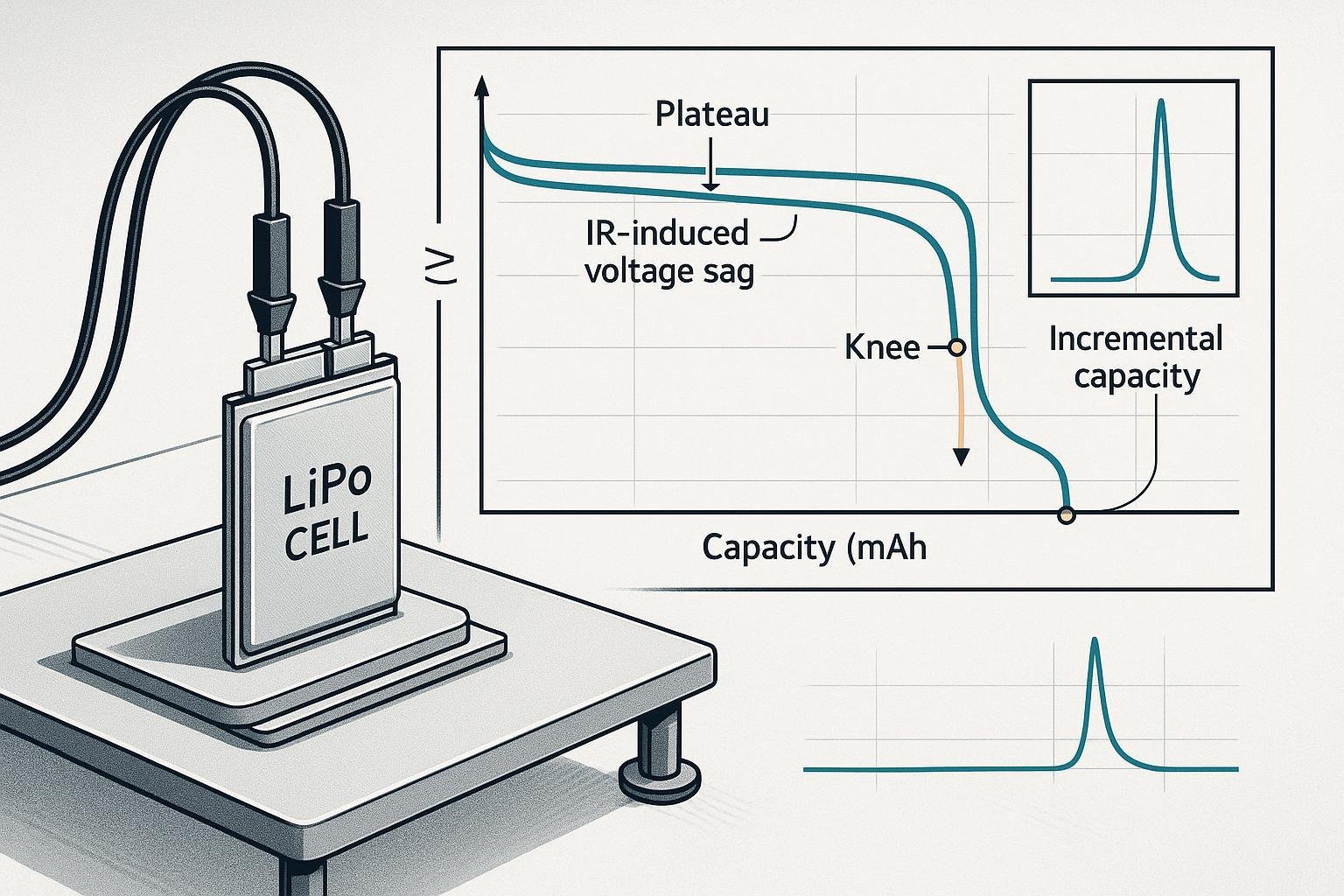
2) Read the curve like a pro: what each feature means and how to verify

A standard discharge curve (V vs. Q or V vs. time at constant current) contains recurring landmarks. Here’s how to interpret them and what to do next.

• Plateau slope (mid‑SOC region)

  • What it means: A steeper slope compared with beginning‑of‑life (BOL) indicates increased polarization and/or loss of active sites.
  • Verify: Compare to your 25 °C reference, keeping the C‑rate constant. If slope steepening correlates with colder tests or higher rates, it may be a reversible condition, not aging. See interpretive examples in plateau and slope behavior — Biologic Learning Center (2024).
  • Act: If steepening persists at reference conditions, schedule an IR pulse test and a low‑rate diagnostic discharge (see ICA/DVA below).

• Voltage sag under load (instant drop when current is applied)

  • What it means: IR and concentration polarization; sag grows with current and lower temperatures. Growth over life usually tracks rising impedance.
  • Verify: Use short current pulses with high‑rate logging to estimate dynamic resistance. Temperature‑compensate results. Power capability workflows build on this principle in USABC/INL protocols; for general context, see NREL FY2022 degradation modeling resource (2022).
  • Act: If sag threatens your minimum operating voltage, derate the load, tighten low‑voltage cutoffs, or qualify cells with lower IR.

• Knee region (pre‑cutoff downturn)

  • What it means: The “knee” typically appears in the last 10–20% SOC at a given C‑rate; aging pushes it earlier and makes the drop steeper.
  • Verify: Compare knee onset (by SOC or delivered Ah) at the same temperature and C‑rate across time. The interpretive method is covered in knee detection on discharge curves — Biologic Learning Center (2024).
  • Act: Implement knee‑onset monitoring in firmware/analytics to warn users earlier or to adjust usable SOC windows.

• End‑of‑discharge (EOD) drop

  • What it means: A sharp terminal decline near cutoff. If it occurs prematurely at moderate loads and normal temperature, expect capacity fade and/or elevated impedance.
  • Verify: Cross‑check with a low‑rate capacity test at 25 °C. If early EOD persists, run a pulse IR test and ICA/DVA to separate loss mechanisms.
  • Act: Increase safety margins on cutoff voltage for high‑load or cold scenarios; review cell matching in packs.

• Voltage recovery and hysteresis (after load removal)

  • What it means: Voltage rebounds as gradients relax; larger rebound and wider charge‑discharge hysteresis suggest higher polarization or low‑temperature operation.
  • Verify: Compare recovery magnitude/time constants at the same SOC and temperature. Practical guidance appears in voltage recovery and hysteresis discussion — Biologic Learning Center (2024).
  • Act: If recovery is large in normal conditions, investigate cooling, current spikes, or contact resistance; consider pre‑warming in cold operations.

3) Advanced diagnostics from the same discharge: ICA/DVA to pinpoint degradation modes

When basic features signal trouble, run a low‑rate diagnostic to extract higher‑value features.

Recommended profile

• Charge CCCV under temperature control; rest adequately.
• Discharge at C/10 (or lower) to the specified cutoff. Record high‑resolution V–Q.

Preprocessing and differentiation

• Smooth Q–V with a conservative filter (e.g., Savitzky–Golay) to reduce noise, then compute dQ/dV (Incremental Capacity Analysis, ICA) and/or dV/dQ (Differential Voltage Analysis, DVA). Over‑smoothing erases diagnostic peaks; tune on a BOL reference. The rationale for derivative‑based interpretation is treated in derivative features on cycling curves — Biologic Learning Center (2024).

Interpreting the peaks (quick guide)

• Loss of Lithium Inventory (LLI): peak positions shift (capacity‑axis) with shapes relatively preserved.
• Loss of Active Material (LAM): peak heights/areas reduce and shapes alter, indicating fewer active sites.

Actions based on ICA/DVA

• Predominant LLI: Expect reduced voltage headroom and earlier knee; adjust charging protocols if appropriate and re‑evaluate cutoff margins.
• Predominant LAM: Plan for irreversible capacity loss; review mechanical integrity and cycling stress.

Why this matters in 2025

• While EIS can separate kinetics more cleanly, discharge‑derived ICA/DVA still offers high diagnostic value in labs without impedance analyzers, and can be automated. For complementary future‑leaning methods, see 2025 work on edge models using electrochemical impedance in TinyML SoH estimation based on EIS — ScienceDirect (2025).

4) Normalize for temperature and C‑rate before you call it “aging”

Temperature and load confound nearly every discharge feature. Normalize or test across a matrix to avoid mislabeling reversible effects.

A pragmatic normalization workflow

1. Define a reference point (25 °C, 0.2–0.5C) and always include it in test sets.
2. Add a small matrix: e.g., 0/10/25/40 °C × 0.2C/1C/2C. This separates reversible thermal‑rate effects from permanent degradation.
3. Compare like with like: only judge slope/knee/EOD vs. BOL at the same condition.
4. Use simple temperature compensation for IR and OCV where available; record ambient and cell temperatures in every session.

Open tools and data to help

• NREL provides models, datasets, and code to study temperature and current impacts on performance and life. See the NREL BLAST portal and the open BLAST‑Lite modeling code on GitHub (maintained 2022–2025). Broader data governance and lifetime modeling guidance is documented in the NREL FY2022 degradation modeling resource and the NREL FY2024 data and lifetime report.

What not to do

• Don’t compare a 0 °C, 1C discharge curve to a 25 °C, 0.5C BOL curve and call it “aging.” That’s temperature/kinetics, not necessarily degradation.

5) Efficiency you can measure from discharge data

Two efficiency metrics matter in practice.

• Coulombic efficiency (CE)

  • CE = discharged Ah / charged Ah across a full cycle. In healthy Li‑ion cycling under benign conditions, CE is typically >99.5%, so deviations are a red flag—though you should average multiple cycles to reduce noise. See definitions and practical ranges in SoC/SoH fundamentals — Biologic Learning Center (2024).

• Energy efficiency

  • Ratio of discharged Wh to charged Wh. Track alongside voltage‑plateau shifts and IR growth; higher current and lower temperatures reduce this metric as polarization losses grow. Use the same temperature/load normalization principles as above.

How to use efficiency trends

• If CE trends down while IR remains steady, suspect side reactions or data/measurement issues. If energy efficiency falls mainly at high rate/cold, focus on impedance growth and thermal conditioning.

6) Embedding discharge‑curve analytics in QA and BMS

You’ll get the most value by standardizing a minimal set of offline tests and complementing it with online analytics.

Offline QA (cell or pack acceptance)

• Always run a reference capacity discharge at 25 °C and moderate C‑rate.
• Add a short pulse sequence (or HPPC) to estimate dynamic IR across several SOC rungs; archive raw curves. NREL’s reports provide context for power‑capability characterization and analysis workflows; see the NREL FY2024 data and lifetime report.
• For suspect lots, schedule a low‑rate ICA/DVA session to identify LLI vs. LAM tendencies.

Online/BMS or field analytics

• Enhance coulomb counting with voltage‑vs‑capacity fingerprints learned at reference conditions, updated opportunistically during partial discharges. Industry practice combining voltage fingerprints and temperature correction is outlined in Analog Devices — SoC/SoH estimation practices (2023–2024).
• Knee early‑warning: track dV/dQ or dV/dt slopes at recurring operating points; alert when knee onset shifts earlier by a configured threshold.
• Opportunistic IR tracking: estimate dynamic resistance from natural load transients, temperature‑correct, and trend over time.
• Data governance: decimate routine data but keep high‑resolution snippets around transients and EOD events. Persist calibration and environment metadata, per guidance in the NREL FY2024 battery data governance report.

7) Troubleshooting patterns you can spot in minutes

• Excessive voltage sag at moderate current vs. BOL

  • Likely cause: IR rise (SEI growth, contact resistance) or cold operation.
  • What to do: Validate wiring/contacts; run a pulse IR test; temperature‑correct; consider derating.

• Early knee onset and reduced delivered capacity at reference conditions

  • Likely cause: capacity fade and/or impedance growth.
  • What to do: Run ICA/DVA to separate LLI vs. LAM signatures; adjust usable SOC; review cycling and thermal history.

• Irregular end‑of‑discharge behavior across parallel cells in a pack

  • Likely cause: cell imbalance or mismatch.
  • What to do: Audit pack balancing; perform controlled full charges; compare per‑cell curves.

• Large voltage recovery and widened hysteresis after load removal

  • Likely cause: high polarization from high C‑rate or low temperature.
  • What to do: Reduce peak load, pre‑warm cells, or retune thermal management.

• Apparent CE below expected range but no corroborating signs of degradation

  • Likely cause: measurement noise, timing drift, or logging gaps.
  • What to do: Recalibrate instruments, verify timebase, and average multiple cycles; see data‑quality practices in the NREL FY2024 data and lifetime report.

8) Boundaries and trade‑offs: where discharge curves excel and where they don’t

• No single curve feature uniquely identifies a degradation mode. Triangulate: capacity at reference, IR/pulse power, and (when available) ICA/DVA. For broader lifetime modeling context and variable interactions, see NREL FY2022 degradation modeling resource.
• Temperature and load can impersonate aging. If you cannot control them, log them rigorously and normalize. The BLAST family’s public materials illustrate how temperature/SOC/current interact; see the NREL BLAST portal.
• Automation pitfalls: numerical differentiation amplifies noise; tune filters against a BOL reference and validate on multiple samples. Watch for domain shift when applying models trained at narrow operating ranges; maintain fallbacks. These cautions align with data‑quality guidance in the NREL FY2024 battery data governance report.

9) What’s next: complementing discharge curves with EIS and edge intelligence

Discharge curves will remain your backbone because they’re easy to collect at scale and directly tied to usable energy and voltage limits. But you can add two layers as budgets allow:

• Impedance features via EIS (offline or in situ): help separate kinetic mechanisms underlying sag and hysteresis. Recent 2025 work demonstrates on‑device feasibility for SoH using compact models on EIS features, as reported in TinyML SoH estimation based on EIS — ScienceDirect (2025).

• Cloud/edge analytics on curve features: compress segments (plateau slopes, knee indices, recovery magnitudes) at the edge and periodically sync to backends trained on reference conditions, following governance principles like those in the NREL FY2024 data and lifetime report.

Quick start: a 90‑minute diagnostic you can run this week

• Prepare a single cell, environmental chamber at 25 °C, and a calibrated cycler.
• Charge CCCV to full; rest 45 minutes.
• Discharge at 0.5C to cutoff; log at 5 Hz with a 5‑second 1C pulse at 80%, 50%, and 20% SOC.
• Plot V–Q and annotate: mid‑plateau slope, knee onset (SOC), EOD drop sharpness, pulse‑sag values.
• If anomalies are present, schedule a C/10 diagnostic discharge for ICA/DVA next session.
• File curves and metadata into your QA repository per the NREL FY2024 governance recommendations.

Key takeaways

• Control temperature and C‑rate or normalize rigorously; otherwise you’ll confuse reversible effects with aging.
• Read the whole curve: slope, sag, knee, EOD drop, and recovery together tell a coherent story.
• Use ICA/DVA at low rate to separate LLI vs. LAM when capacity fades.
• Trend IR and knee onset in QA/BMS; combine with voltage‑fingerprint SoH for robust field estimation.
• Maintain data hygiene: synchronized V/I/T/time, calibration logs, and test metadata.

References and further reading

• Practical interpretation of discharge features and curve types: Biologic Learning Center — how to read cycling curves (2024)
• Definitions and efficiency ranges: Biologic Learning Center — SoC/SoH fundamentals (2024)
• Temperature/rate interactions, lifetime modeling, and data governance: NREL BLAST portal; NREL FY2022 degradation modeling resource; NREL FY2024 battery data and lifetime report
• SoC/SoH estimation in embedded systems: Analog Devices — SoC/SoH estimation practices (2023–2024)
• Complementary advanced method trend: TinyML SoH estimation based on EIS — ScienceDirect (2025)